The loss function used for the training of Variational Autoencoders (VAEs) is divided in two terms. The first one measures the quality of the autoencoding, i.e. the error between the original sample and its reconstruction. The second term is the Kullback-Leibler divergence (abbreviated KL divergence) with respect to a standard multivariate normal distribution. We will illustrate with a few plots the influence of the KL divergence on the encoder and decoder outputs.
A short introduction to building autoencoders is available on the Keras blog. Multiple autoencoders are presented, the last one being the Variational Autoencoder. If you don’t know what is a VAE, you could start by giving a look at that introduction.
The purpose of the KL divergence term in the loss function is to make the distribution of the encoder output as close as possible to a standard multivariate normal distribution. In the following, we will consider an autoencoder with a latent space of dimension 2. As a reference, let’s first plot points sampled from the standard multivariate normal distribution in the two-dimensional case.
%matplotlib inline
import numpy as np
import matplotlib.pyplot as plt

plt.figure(figsize=(12, 10))
z = np.random.multivariate_normal([0] * 2, np.eye(2), 5000)
plt.scatter(z[:, 0], z[:, 1])
plt.xlabel("z[0]")
plt.ylabel("z[1]")
plt.title('Samples from a 2D standard multivariate normal distribution')
plt.show()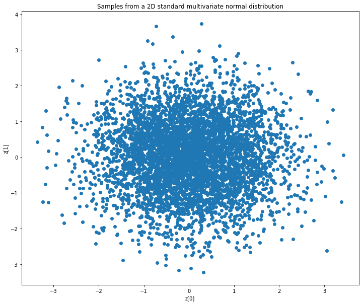
The ideal output of our encoder would look similar to the above plot.
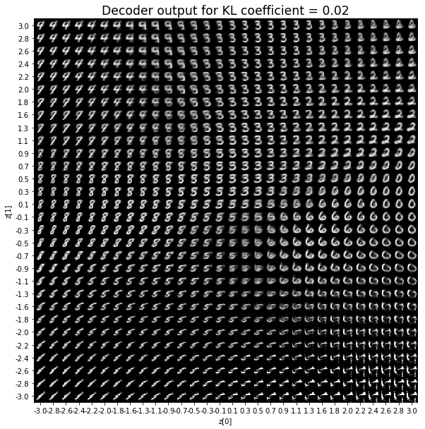
In the following, we will modify the Variational Autoencoder example from the Keras repository to show how the KL divergence influence both the encoder and decoder ouputs. We add a coefficient \(c\) to the KL divergence. The loss function therefore becomes loss = reconstruction_loss + c * kl_loss. We look at the result for different values of \(c\).
'''Example showing the influence of the KL divergence on the encoder and
decoder ouputs.
This is a modification of Keras VAE example that is available at:
https://github.com/keras-team/keras/blob/master/examples/variational_autoencoder.py
'''
from keras.layers import Lambda, Input, Dense
from keras.models import Model
from keras.datasets import mnist
from keras.losses import binary_crossentropy
from keras.optimizers import Adam
from keras import backend as K
import numpy as np
import matplotlib.pyplot as plt
from tqdm import tqdm
# reparameterization trick
# instead of sampling from Q(z|X), sample epsilon = N(0,I)
# z = z_mean + sqrt(var) * epsilon
def sampling(args):
"""Reparameterization trick by sampling from an isotropic unit Gaussian.
# Arguments
args (tensor): mean and log of variance of Q(z|X)
# Returns
z (tensor): sampled latent vector
"""
z_mean, z_log_var = args
batch = K.shape(z_mean)[0]
dim = K.int_shape(z_mean)[1]
# by default, random_normal has mean = 0 and std = 1.0
epsilon = K.random_normal(shape=(batch, dim))
return z_mean + K.exp(0.5 * z_log_var) * epsilon
def plot_results(models,
data,
kl_coefficient,
batch_size=128):
"""Plots labels and MNIST digits as a function of the 2D latent vector
# Arguments
models (tuple): encoder and decoder models
data (tuple): test data and label
batch_size (int): prediction batch size
kl_coefficient (double): the KL loss coefficient
"""
encoder, decoder = models
x_test, y_test = data
# display a 2D plot of the digit classes in the latent space
z_mean, _, _ = encoder.predict(x_test,
batch_size=batch_size)
plt.figure(figsize=(12, 10))
plt.scatter(z_mean[:, 0], z_mean[:, 1], c=y_test)
plt.colorbar()
plt.xlabel("z[0]")
plt.ylabel("z[1]")
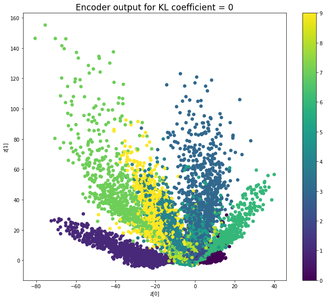
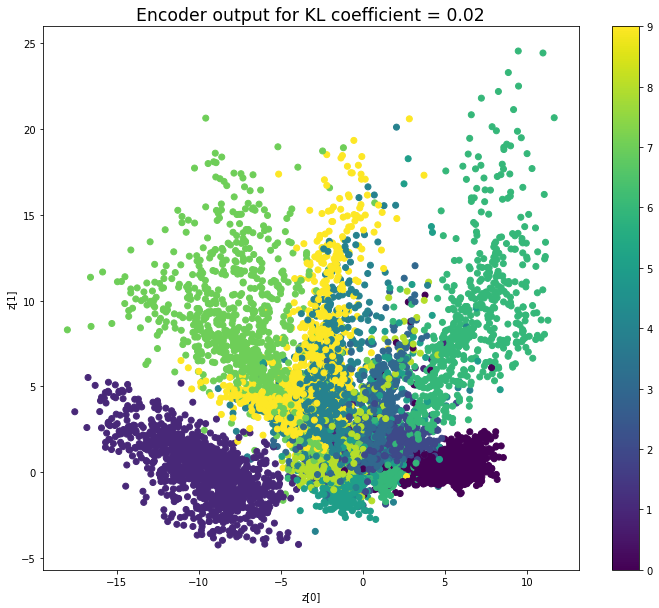
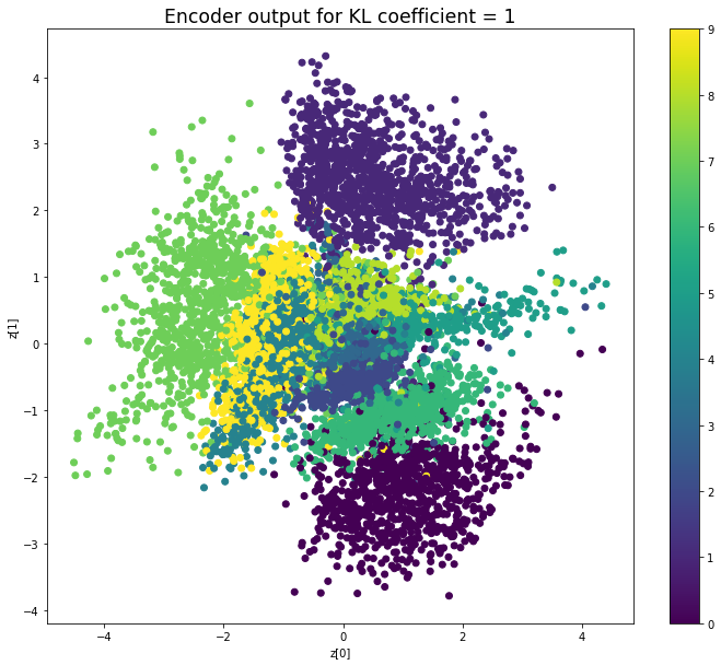
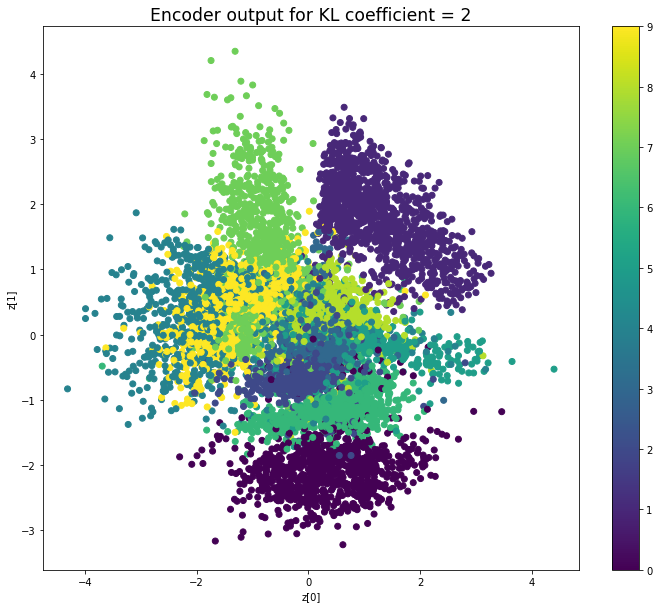
plt.title(f'Encoder output for KL coefficient = {kl_coefficient}', fontdict={'fontsize': 'xx-large'})
plt.show()
print('\n')
# display a 30x30 2D manifold of digits
n = 30
digit_size = 28
figure = np.zeros((digit_size * n, digit_size * n))
# linearly spaced coordinates corresponding to the 2D plot
# of digit classes in the latent space
grid_x = np.linspace(-3, 3, n)
grid_y = np.linspace(-3, 3, n)[::-1]
for i, yi in enumerate(grid_y):
for j, xi in enumerate(grid_x):
z_sample = np.array([[xi, yi]])
x_decoded = decoder.predict(z_sample)
digit = x_decoded[0].reshape(digit_size, digit_size)
figure[i * digit_size: (i + 1) * digit_size,
j * digit_size: (j + 1) * digit_size] = digit
plt.figure(figsize=(10, 10))
start_range = digit_size // 2
end_range = (n - 1) * digit_size + start_range + 1
pixel_range = np.arange(start_range, end_range, digit_size)
sample_range_x = np.round(grid_x, 1)
sample_range_y = np.round(grid_y, 1)
plt.xticks(pixel_range, sample_range_x)
plt.yticks(pixel_range, sample_range_y)
plt.xlabel("z[0]")
plt.ylabel("z[1]")
plt.imshow(figure, cmap='Greys_r')
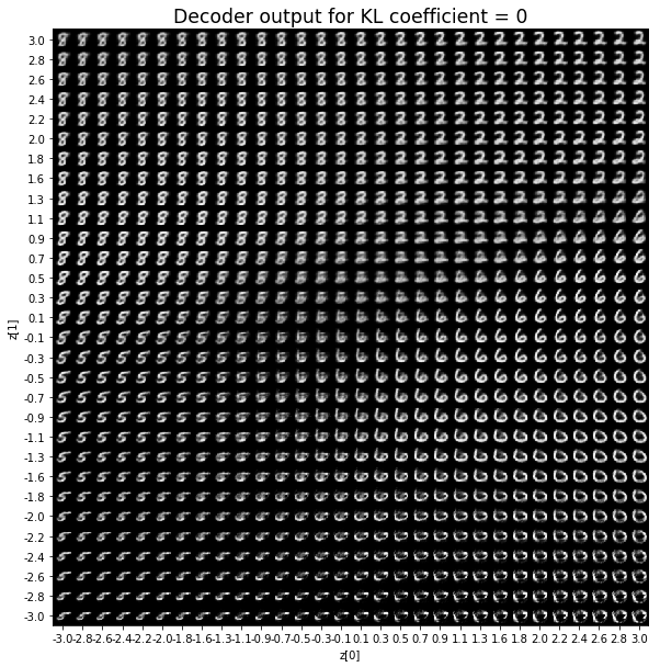
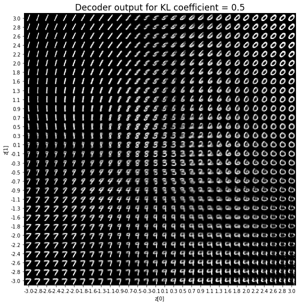
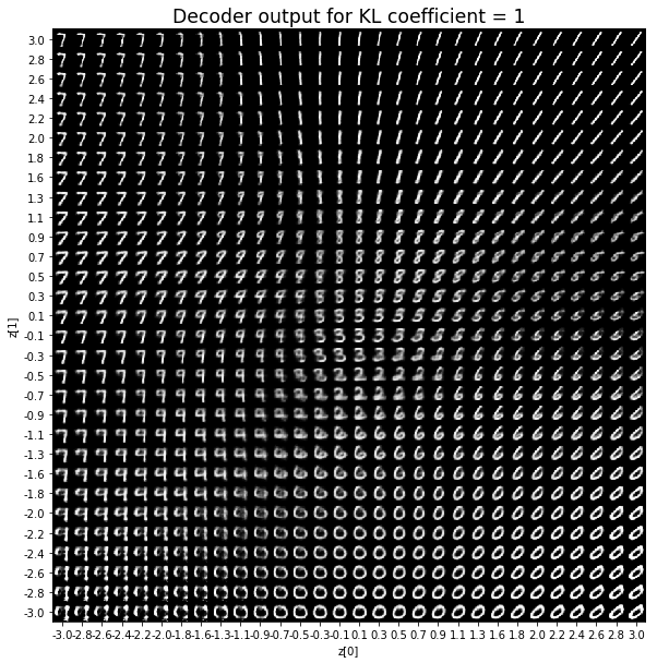
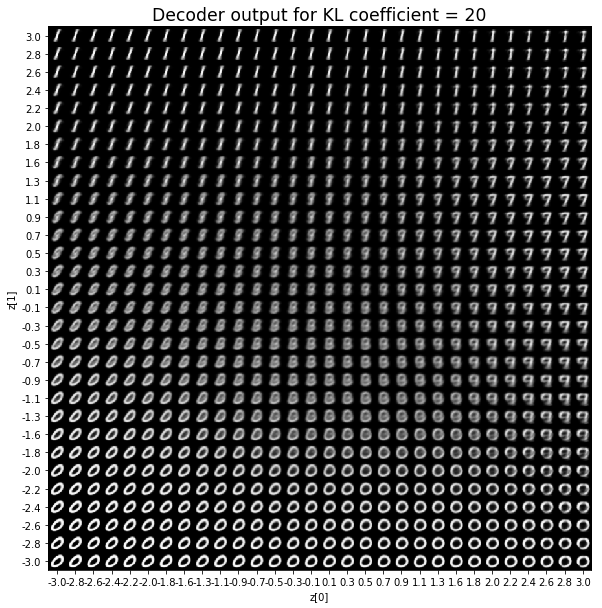
plt.title(f'Decoder output for KL coefficient = {kl_coefficient}', fontdict={'fontsize': 'xx-large'})
plt.show()
def build_model(input_shape, intermediate_dim, latent_dim, original_dim):
# VAE model = encoder + decoder
# build encoder model
inputs = Input(shape=input_shape, name='encoder_input')
x = Dense(intermediate_dim, activation='relu')(inputs)
z_mean = Dense(latent_dim, name='z_mean')(x)
z_log_var = Dense(latent_dim, name='z_log_var')(x)
# use reparameterization trick to push the sampling out as input
# note that "output_shape" isn't necessary with the TensorFlow backend
z = Lambda(sampling, output_shape=(latent_dim,), name='z')([z_mean, z_log_var])
# instantiate encoder model
encoder = Model(inputs, [z_mean, z_log_var, z], name='encoder')
# build decoder model
latent_inputs = Input(shape=(latent_dim,), name='z_sampling')
x = Dense(intermediate_dim, activation='relu')(latent_inputs)
outputs = Dense(original_dim, activation='sigmoid')(x)
# instantiate decoder model
decoder = Model(latent_inputs, outputs, name='decoder')
# instantiate VAE model
outputs = decoder(encoder(inputs)[2])
vae = Model(inputs, outputs, name='vae_mlp')
models = (encoder, decoder)
reconstruction_loss = binary_crossentropy(inputs, outputs)
reconstruction_loss *= original_dim
reconstruction_loss = K.mean(reconstruction_loss)
kl_loss = 1 + z_log_var - K.square(z_mean) - K.exp(z_log_var)
kl_loss = K.sum(kl_loss, axis=-1)
kl_loss *= -0.5
kl_loss = K.mean(kl_loss)
return vae, models, reconstruction_loss, kl_loss
# MNIST dataset
(x_train, y_train), (x_test, y_test) = mnist.load_data()
image_size = x_train.shape[1]
original_dim = image_size * image_size
x_train = np.reshape(x_train, [-1, original_dim])
x_test = np.reshape(x_test, [-1, original_dim])
x_train = x_train.astype('float32') / 255
x_test = x_test.astype('float32') / 255
# network parameters
input_shape = (original_dim, )
intermediate_dim = 512
batch_size = 128
latent_dim = 2
epochs = 40
data = (x_test, y_test)
vae, _, _, _ = build_model(input_shape, intermediate_dim, latent_dim, original_dim)
vae.save_weights('vae_init.h5')
for kl_coefficient in [0, 0.02, 0.1, 0.5, 1, 2, 10, 20]:
print('—' * 80)
print('KL coefficient:', kl_coefficient, flush=True)
vae, models, reconstruction_loss, kl_loss = build_model(input_shape, intermediate_dim, latent_dim, original_dim)
vae.load_weights('vae_init.h5')
vae_loss = reconstruction_loss + kl_coefficient * kl_loss
vae.add_loss(vae_loss)
vae.compile(optimizer=Adam(lr=1e-3))
vae.metrics_tensors.append(reconstruction_loss)
vae.metrics_names.append("reconstruct")
vae.metrics_tensors.append(kl_loss)
vae.metrics_names.append("kl")
for epoch in tqdm(range(epochs), desc='Training'):
vae.fit(x_train,
epochs=1,
batch_size=batch_size,
verbose=0)
test_losses = vae.evaluate(data[0], verbose=0)
print(f'Test loss: {test_losses[0]}, Reconstruction loss: {test_losses[1]}, KL loss: {test_losses[2]}')
plot_results(models, data, kl_coefficient, batch_size)
Using TensorFlow backend.


————————————————————————————————————————————————————————————————————————————————
KL coefficient: 0


Training: 100%|██████████| 40/40 [01:00<00:00,  1.47s/it]


Test loss: 141.54102014160156, Reconstruction loss: 141.54102014160156, KL loss: 506.81957373046873
————————————————————————————————————————————————————————————————————————————————
KL coefficient: 0.02


Training: 100%|██████████| 40/40 [01:00<00:00,  1.48s/it]


Test loss: 143.99177861328124, Reconstruction loss: 143.37973349609376, KL loss: 30.602262100219725
————————————————————————————————————————————————————————————————————————————————
KL coefficient: 0.1


Training: 100%|██████████| 40/40 [01:01<00:00,  1.49s/it]


Test loss: 142.62690827636717, Reconstruction loss: 141.40527036132812, KL loss: 12.216379901123046
————————————————————————————————————————————————————————————————————————————————
KL coefficient: 0.5


Training: 100%|██████████| 40/40 [01:01<00:00,  1.50s/it]


Test loss: 147.35851181640626, Reconstruction loss: 143.7733653808594, KL loss: 7.170292739105225
————————————————————————————————————————————————————————————————————————————————
KL coefficient: 1


Training: 100%|██████████| 40/40 [01:02<00:00,  1.53s/it]


Test loss: 150.38663830566406, Reconstruction loss: 144.17457075195313, KL loss: 6.21206757888794
————————————————————————————————————————————————————————————————————————————————
KL coefficient: 2


Training: 100%|██████████| 40/40 [01:02<00:00,  1.54s/it]


Test loss: 156.17380212402344, Reconstruction loss: 145.99718872070312, KL loss: 5.088306475830078
————————————————————————————————————————————————————————————————————————————————
KL coefficient: 10


Training: 100%|██████████| 40/40 [01:03<00:00,  1.58s/it]


Test loss: 186.47321110839843, Reconstruction loss: 161.8455504638672, KL loss: 2.4627660331726076
————————————————————————————————————————————————————————————————————————————————
KL coefficient: 20


Training: 100%|██████████| 40/40 [01:04<00:00,  1.57s/it]


Test loss: 203.30997185058592, Reconstruction loss: 189.7224153808594, KL loss: 0.6793778092384338
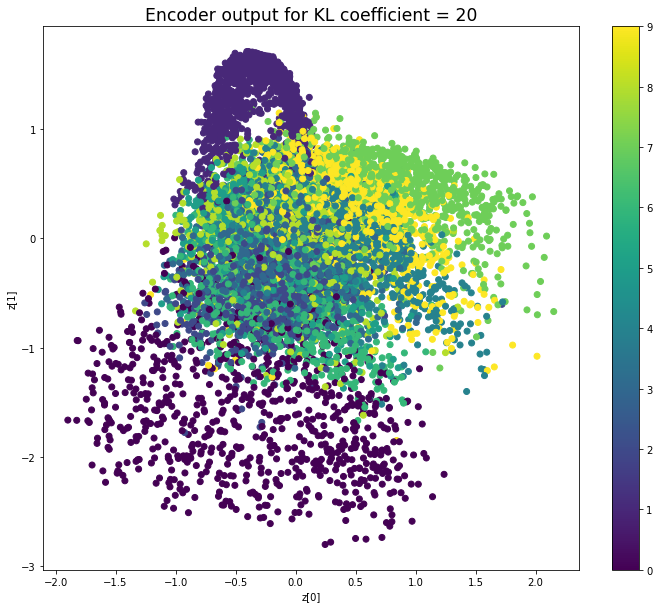
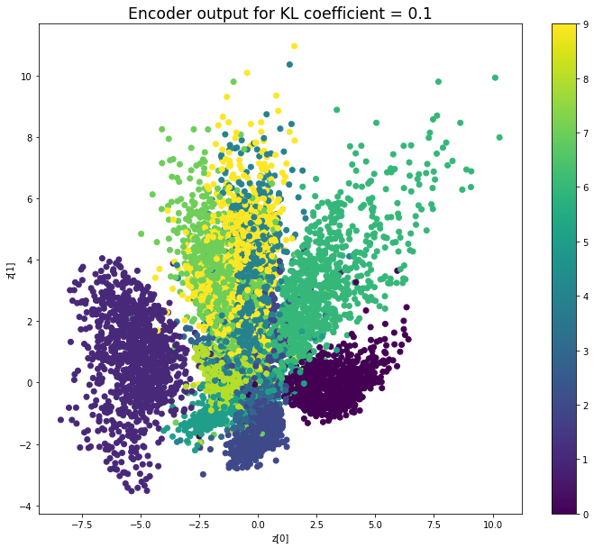
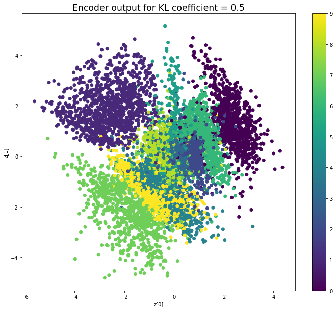
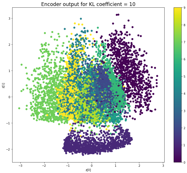
When the KL loss is not used (coefficient = 0), the output values of the encoder are really scattered. When increasing the coefficient, the values start to gather around the origin. While far from being perfect, we see that a correctly chosen coefficient helps to get a result closer to the reference plot of the 2D standard multivariate normal distribution.
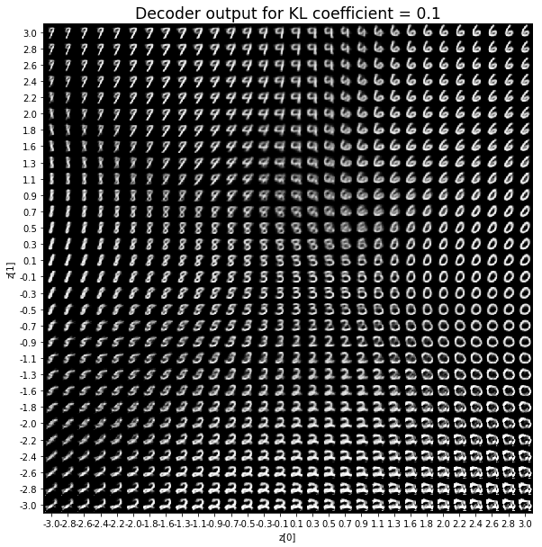
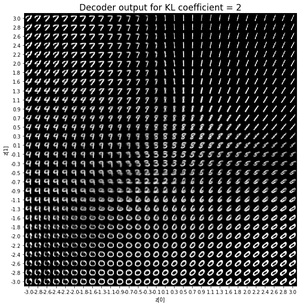
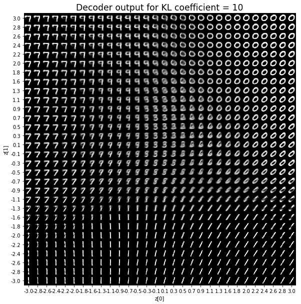
As for the decoder output, a big coefficient gives a result with many blurry values and only a few digits. A very small coefficient doesn’t seem to generate all the digits either.
Overall, average coefficients such as 0.5, 1 and 2 seem to provide the best result.
In the previous example, choosing equal weights for the reconstruction loss and the KL loss leads to good results. However, be careful, this may depend on the problem studied as well as how you define your losses. For example, the above reconstruction loss is defined as image_dim * binary_crossentropy, not as binary_crossentropy.