We saw in a previous post how the Kullback-Leibler divergence influence a VAE’s encoder and decoder outputs. In particular, we could notice that whereas the encoder outputs are closer to a standard multivariate normal distribution thanks to the KL divergence, the result is far from being perfect and there are still some gaps. The Adversarial Autoencoder tends to fix that problem by using a Generative Adversarial Network rather than the KL divergence.
To learn in details what are Adversarial Autoencoders, you can read the original paper. In the following, we modified the code of the post On the use of the Kullback–Leibler divergence in Variational Autoencoders, replacing the VAE by an AAE. We will plot the encoder and decoder outputs every 10 epochs, over a training of 100 epochs.
'''Example showing the convergence of an adversarial autoencoder.
We modified the code from the post "On the use of the Kullback-Leibler divergence in VAEs"
'''
%matplotlib inline
from keras.layers import Input, Dense
from keras.models import Model
from keras.datasets import mnist
from keras.losses import binary_crossentropy
from keras.optimizers import Adam
import numpy as np
import matplotlib.pyplot as plt
def plot_results(encoder,
decoder,
data,
batch_size=128):
"""Plots labels and MNIST digits as a function of the 2D latent vector
# Arguments
encoder: encoder model
decoder: decoder model
data (tuple): test data and label
batch_size (int): prediction batch size
"""
x_test, y_test = data
# display a 2D plot of the digit classes in the latent space
z_mean = encoder.predict(x_test,
batch_size=batch_size)
plt.figure(figsize=(12, 10))
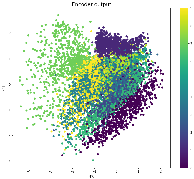
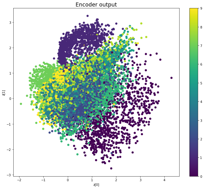
plt.scatter(z_mean[:, 0], z_mean[:, 1], c=y_test)
plt.colorbar()
plt.xlabel("z[0]")
plt.ylabel("z[1]")
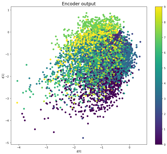
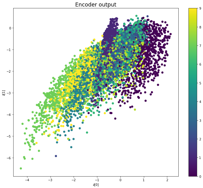
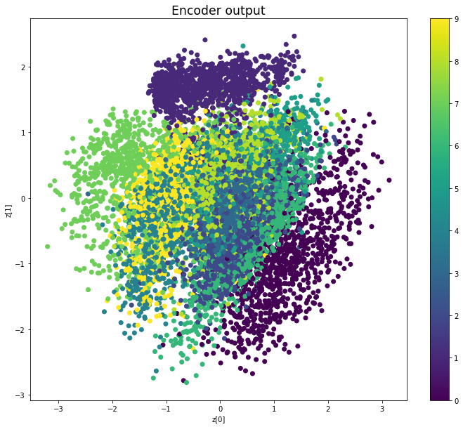
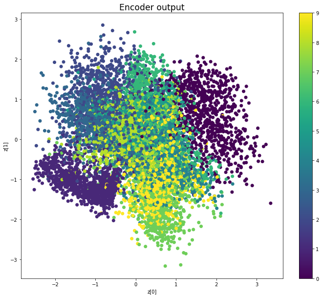
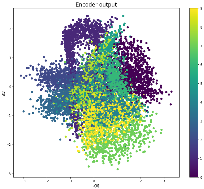
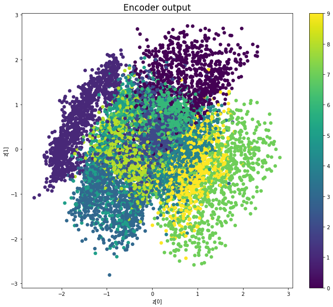
plt.title(f'Encoder output', fontdict={'fontsize': 'xx-large'})
plt.show()
print('\n')
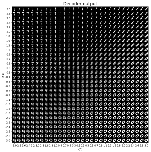
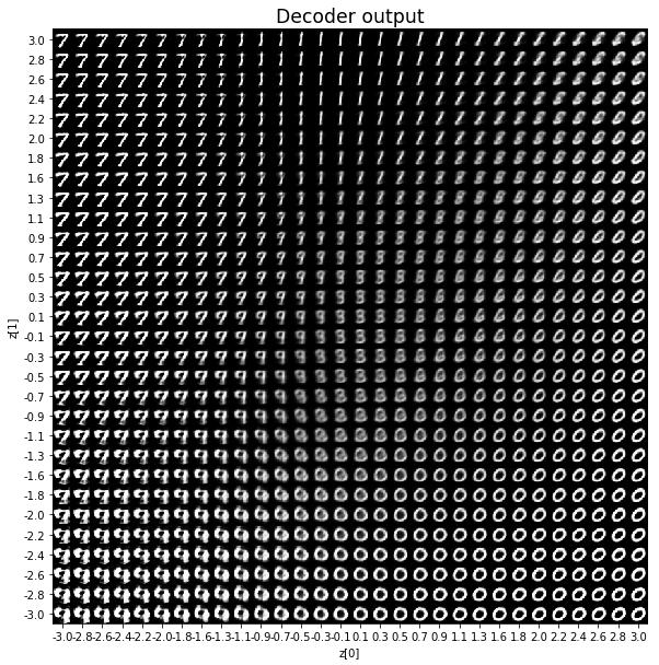
# display a 30x30 2D manifold of digits
n = 30
digit_size = 28
figure = np.zeros((digit_size * n, digit_size * n))
# linearly spaced coordinates corresponding to the 2D plot
# of digit classes in the latent space
grid_x = np.linspace(-3, 3, n)
grid_y = np.linspace(-3, 3, n)[::-1]
for i, yi in enumerate(grid_y):
for j, xi in enumerate(grid_x):
z_sample = np.array([[xi, yi]])
x_decoded = decoder.predict(z_sample)
digit = x_decoded[0].reshape(digit_size, digit_size)
figure[i * digit_size: (i + 1) * digit_size,
j * digit_size: (j + 1) * digit_size] = digit
plt.figure(figsize=(10, 10))
start_range = digit_size // 2
end_range = (n - 1) * digit_size + start_range + 1
pixel_range = np.arange(start_range, end_range, digit_size)
sample_range_x = np.round(grid_x, 1)
sample_range_y = np.round(grid_y, 1)
plt.xticks(pixel_range, sample_range_x)
plt.yticks(pixel_range, sample_range_y)
plt.xlabel("z[0]")
plt.ylabel("z[1]")
plt.imshow(figure, cmap='Greys_r')
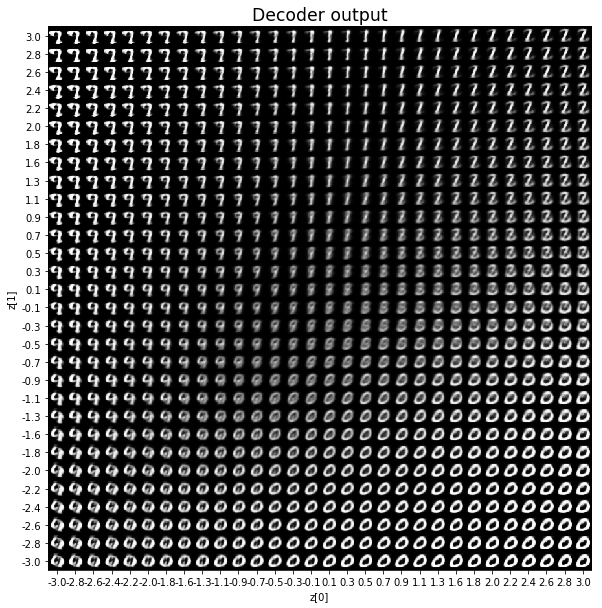
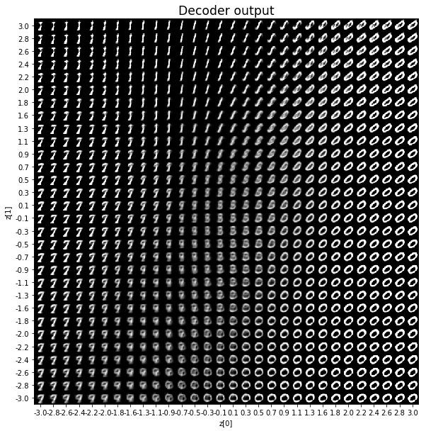
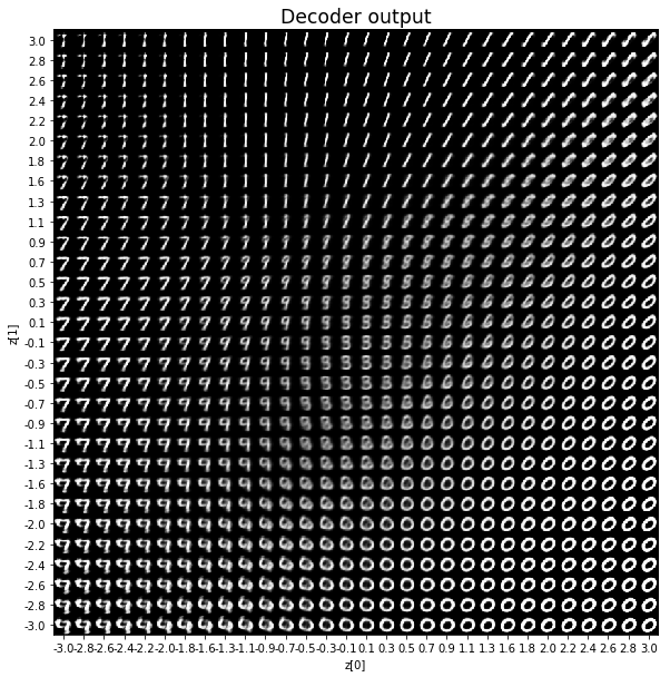
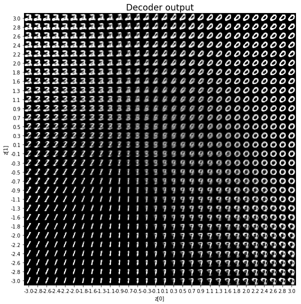
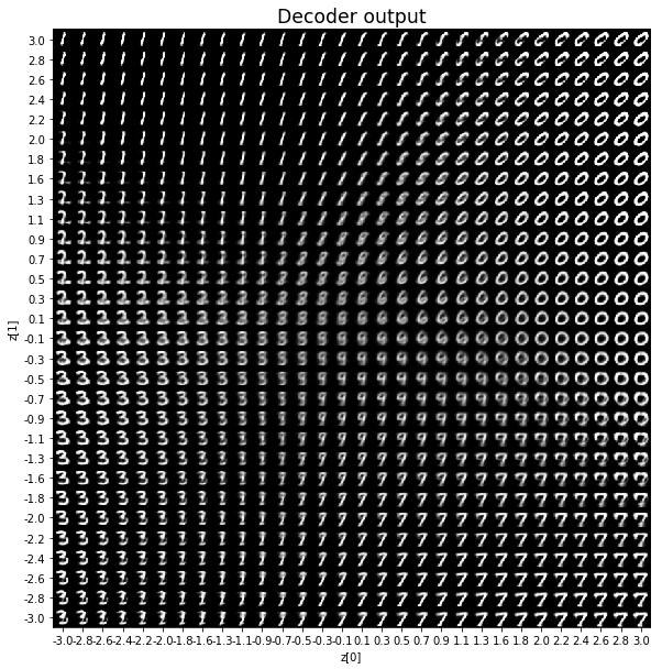
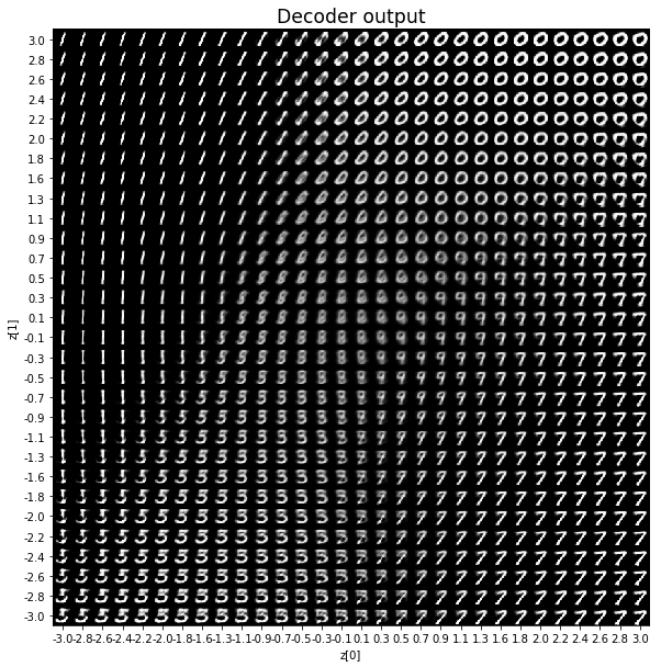
plt.title(f'Decoder output', fontdict={'fontsize': 'xx-large'})
plt.show()
def build_model(input_shape, intermediate_dim, latent_dim, original_dim):
# AAE model = encoder + decoder and generator + discriminator
# build encoder model
inputs = Input(shape=input_shape, name='encoder_input')
x = Dense(intermediate_dim, activation='relu')(inputs)
latent_outputs = Dense(latent_dim)(x)
# instantiate encoder model
encoder = Model(inputs, latent_outputs, name='encoder')
# build decoder model
latent_inputs = Input(shape=(latent_dim,), name='latent_inputs')
x = Dense(intermediate_dim, activation='relu')(latent_inputs)
outputs = Dense(original_dim, activation='sigmoid')(x)
# instantiate decoder model
decoder = Model(latent_inputs, outputs, name='decoder')
# instantiate autoencoder model
outputs = decoder(encoder(inputs))
autoencoder = Model(inputs, outputs, name='aae_mlp')
# build discriminator
x = Dense(intermediate_dim, activation='relu')(latent_inputs)
discriminator_outputs = Dense(1, activation='sigmoid')(x)
discriminator = Model(latent_inputs, discriminator_outputs, name='discriminator')
# build generator
generator_outputs = discriminator(encoder(inputs))
generator = Model(inputs, generator_outputs, name='generator')
models = (encoder, decoder)
autoencoder.compile(optimizer=Adam(lr=1e-3), loss='binary_crossentropy')
for layer in discriminator.layers:
layer.trainable = False
generator.compile(optimizer=Adam(lr=1e-3), loss='binary_crossentropy')
for layer in discriminator.layers:
layer.trainable = True
discriminator.compile(optimizer=Adam(lr=1e-3), loss='binary_crossentropy')
return autoencoder, encoder, decoder, discriminator, generator
# MNIST dataset
(x_train, y_train), (x_test, y_test) = mnist.load_data()
image_size = x_train.shape[1]
original_dim = image_size * image_size
x_train = np.reshape(x_train, [-1, original_dim])
x_test = np.reshape(x_test, [-1, original_dim])
x_train = x_train.astype('float32') / 255
x_test = x_test.astype('float32') / 255
# network parameters
input_shape = (original_dim, )
intermediate_dim = 512
batch_size = 128
latent_dim = 2
epochs = 100
data = (x_test, y_test)
aae, encoder, decoder, discriminator, generator = build_model(input_shape, intermediate_dim, latent_dim, original_dim)
print('—' * 80)
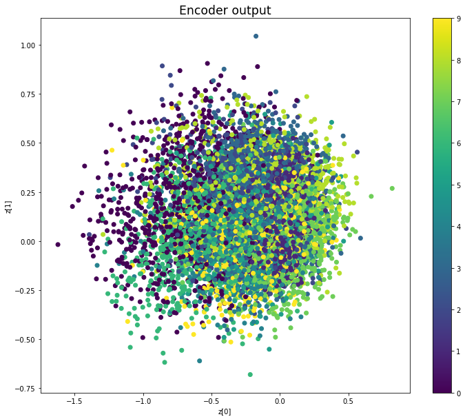
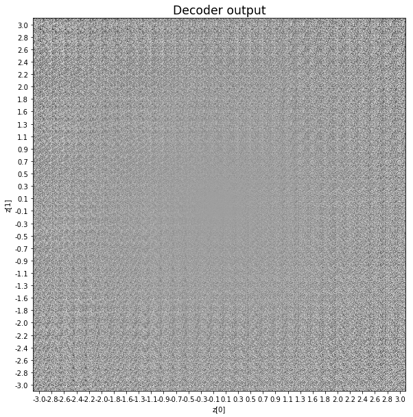
print('Before training')
plot_results(encoder, decoder, data, batch_size)
for epoch in range(epochs):
for n_batch in range(len(x_train) // batch_size):
# Train autoencoder
indices = np.random.randint(0, x_train.shape[0], batch_size)
x = x_train[indices]
aae.train_on_batch(x, x)
# Train discriminator
indices = np.random.randint(0, x_train.shape[0], batch_size // 2)
encoder_outputs = encoder.predict(x_train[indices])
normal_samples = np.random.multivariate_normal([0] * 2, np.eye(2), batch_size // 2)
x = np.vstack([encoder_outputs, normal_samples])
labels = [0] * (batch_size // 2) + [1] * (batch_size // 2)
for layer in discriminator.layers:
layer.trainable = True
discriminator.train_on_batch(x, labels)
# Train encoder
indices = np.random.randint(0, x_train.shape[0], batch_size)
x = x_train[indices]
labels = [1] * batch_size
for layer in discriminator.layers:
layer.trainable = False
generator.train_on_batch(x, labels)
if epoch % 10 == 9:
print('—' * 80)
print('Epoch:', epoch)
plot_results(encoder, decoder, data, batch_size)
Using TensorFlow backend.


————————————————————————————————————————————————————————————————————————————————
Before training
————————————————————————————————————————————————————————————————————————————————
Epoch: 9
————————————————————————————————————————————————————————————————————————————————
Epoch: 19
————————————————————————————————————————————————————————————————————————————————
Epoch: 29
————————————————————————————————————————————————————————————————————————————————
Epoch: 39
————————————————————————————————————————————————————————————————————————————————
Epoch: 49
————————————————————————————————————————————————————————————————————————————————
Epoch: 59
————————————————————————————————————————————————————————————————————————————————
Epoch: 69
————————————————————————————————————————————————————————————————————————————————
Epoch: 79
————————————————————————————————————————————————————————————————————————————————
Epoch: 89
————————————————————————————————————————————————————————————————————————————————
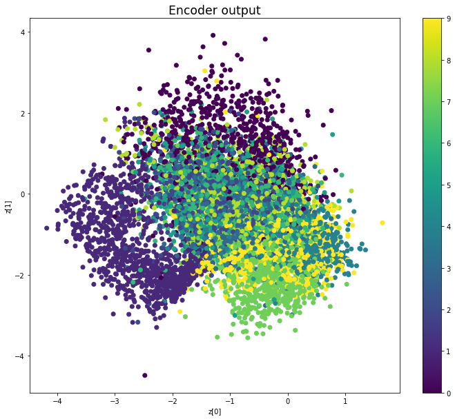
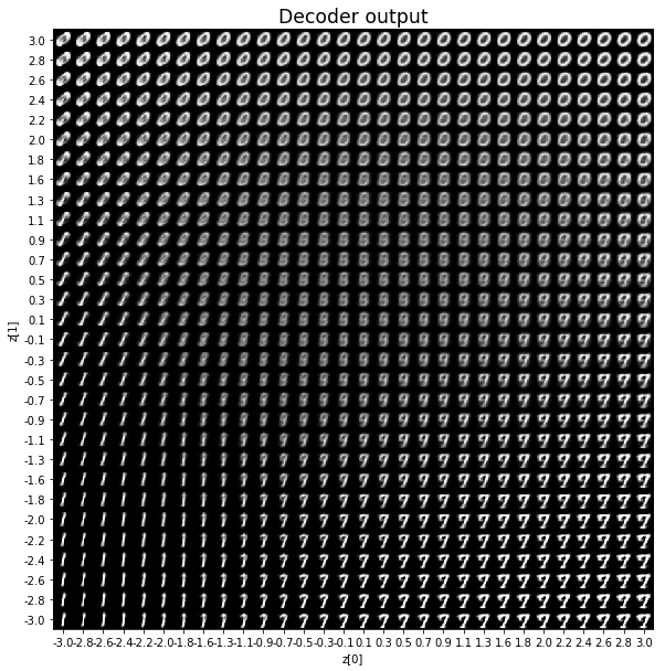
Epoch: 99
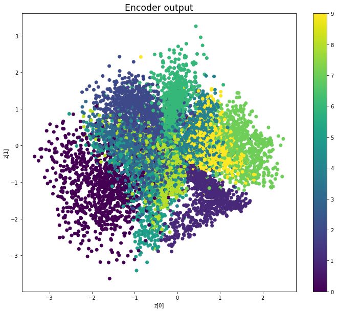
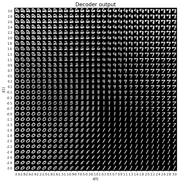
We see that compared to Variational Autoencoders, the encoder outputs of Adversarial Autoencoders are better grouped around 0, with less gaps, and look more like a 2D standard multivariate normal distribution. However, improving the distribution of the encoder outputs has some costs:
- the training of an AAE takes longer than the training of a VAE,
- the training of an AAE is less stable than the training of a VAE.
Indeed, while a VAE requires training only one model, an AAE requires to iteratively train three different models. Having to train three different models at the same time makes it more difficult to find good parameters for convergence.