In this part, we will learn how to profile a CUDA kernel using both nvprof and nvvp, the Visual Profiler. We will use the convolution kernel from Part 3, and discover thanks to profiling how to improve it.
We gathered the code from Part 3 into a file named ‘convolution.py’. Below is its exact content:
with open('convolution.py', 'r') as f:
    print(f.read())
#!/usr/bin/env python3
# -*- coding: utf-8 -*-
from numba import cuda
import numpy as np
import skimage.data
from skimage.color import rgb2gray
from scipy.ndimage.filters import convolve as scipy_convolve
@cuda.jit
def convolve(result, mask, image):
# expects a 2D grid and 2D blocks,
# a mask with odd numbers of rows and columns, (-1-)
# a grayscale image
# (-2-) 2D coordinates of the current thread:
i, j = cuda.grid(2)
# (-3-) if the thread coordinates are outside of the image, we ignore the thread:
image_rows, image_cols = image.shape
if (i >= image_rows) or (j >= image_cols):
return
# To compute the result at coordinates (i, j), we need to use delta_rows rows of the image
# before and after the i_th row,
# as well as delta_cols columns of the image before and after the j_th column:
delta_rows = mask.shape[0] // 2
delta_cols = mask.shape[1] // 2
# The result at coordinates (i, j) is equal to
# sum_{k, l} mask[k, l] * image[i - k + delta_rows, j - l + delta_cols]
# with k and l going through the whole mask array:
s = 0
for k in range(mask.shape[0]):
for l in range(mask.shape[1]):
i_k = i - k + delta_rows
j_l = j - l + delta_cols
# (-4-) Check if (i_k, j_k) coordinates are inside the image:
if (i_k >= 0) and (i_k < image_rows) and (j_l >= 0) and (j_l < image_cols):
s += mask[k, l] * image[i_k, j_l]
result[i, j] = s
if __name__ == '__main__':
# Read image
full_image = rgb2gray(skimage.data.coffee()).astype(np.float32) / 255
image = full_image[150:350, 200:400].copy()
# We preallocate the result array:
result = np.empty_like(image)
# We choose a random mask:
mask = np.random.rand(13, 13).astype(np.float32)
mask /= mask.sum() # We normalize the mask
# We use blocks of 32x32 pixels:
blockdim = (32, 32)
# We compute grid dimensions big enough to cover the whole image:
griddim = (image.shape[0] // blockdim[0] + 1, image.shape[1] // blockdim[1] + 1)
# We apply our convolution to our image:
convolve[griddim, blockdim](result, mask, image)
# We check that the error with respect to Scipy convolve function is small:
scipy_result = scipy_convolve(image, mask, mode='constant', cval=0.0, origin=0)
max_rel_error = np.max(np.abs(result - scipy_result) / np.abs(scipy_result))
if max_rel_error > 1e-5:
raise AssertionError('Maximum relative error w.r.t Scipy convolve is too large: '
+ max_rel_error)
For python files, nvprof can be launched the following way:
nvprof python filename.py
This command executes the default mode of nvprof that is the summary mode.
!nvprof python convolution.py==31134== NVPROF is profiling process 31134, command: python convolution.py
==31134== Profiling application: python convolution.py
==31134== Profiling result:
Type Time(%) Time Calls Avg Min Max Name
GPU activities: 88.56% 420.61us 1 420.61us 420.61us 420.61us cudapy::__main__::convolve$241(Array<float, int=2, C, mutable, aligned>, Array<float, int=2, C, mutable, aligned>, Array<float, int=2, C, mutable, aligned>)
5.89% 27.969us 3 9.3230us 704ns 13.697us [CUDA memcpy HtoD]
5.55% 26.368us 3 8.7890us 704ns 12.832us [CUDA memcpy DtoH]
API calls: 98.23% 117.78ms 1 117.78ms 117.78ms 117.78ms cuDevicePrimaryCtxRetain
0.43% 515.48us 1 515.48us 515.48us 515.48us cuLinkCreate
0.39% 472.98us 3 157.66us 12.402us 419.71us cuMemcpyDtoH
0.28% 334.16us 3 111.39us 10.594us 199.43us cuMemAlloc
0.17% 199.68us 1 199.68us 199.68us 199.68us cuModuleLoadDataEx
0.13% 154.79us 1 154.79us 154.79us 154.79us cuLinkAddData
0.11% 130.80us 1 130.80us 130.80us 130.80us cuLinkComplete
0.11% 128.24us 1 128.24us 128.24us 128.24us cuMemGetInfo
0.07% 87.852us 3 29.284us 13.469us 39.206us cuMemcpyHtoD
0.04% 45.955us 1 45.955us 45.955us 45.955us cuDeviceGetName
0.02% 23.518us 1 23.518us 23.518us 23.518us cuLaunchKernel
0.01% 11.778us 2 5.8890us 725ns 11.053us cuDeviceGet
0.00% 3.1840us 3 1.0610us 353ns 1.6210us cuDeviceGetCount
0.00% 2.9720us 5 594ns 409ns 961ns cuFuncGetAttribute
0.00% 2.0340us 1 2.0340us 2.0340us 2.0340us cuCtxPushCurrent
0.00% 1.4530us 3 484ns 410ns 580ns cuDeviceGetAttribute
0.00% 1.3650us 1 1.3650us 1.3650us 1.3650us cuModuleGetFunction
0.00% 913ns 1 913ns 913ns 913ns cuDeviceComputeCapability
0.00% 880ns 1 880ns 880ns 880ns cuLinkDestroy
nvprof can also be used to collect detailed data that can be next imported into NVIDIA Visual Profiler. We will use the two following commands to create first a timeline and next to collect all the metrics and events:
!nvprof --quiet --export-profile timeline.prof python convolution.py
!nvprof --quiet --metrics all --events all -o metrics-events.prof python convolution.py
We can next launch nvvp:
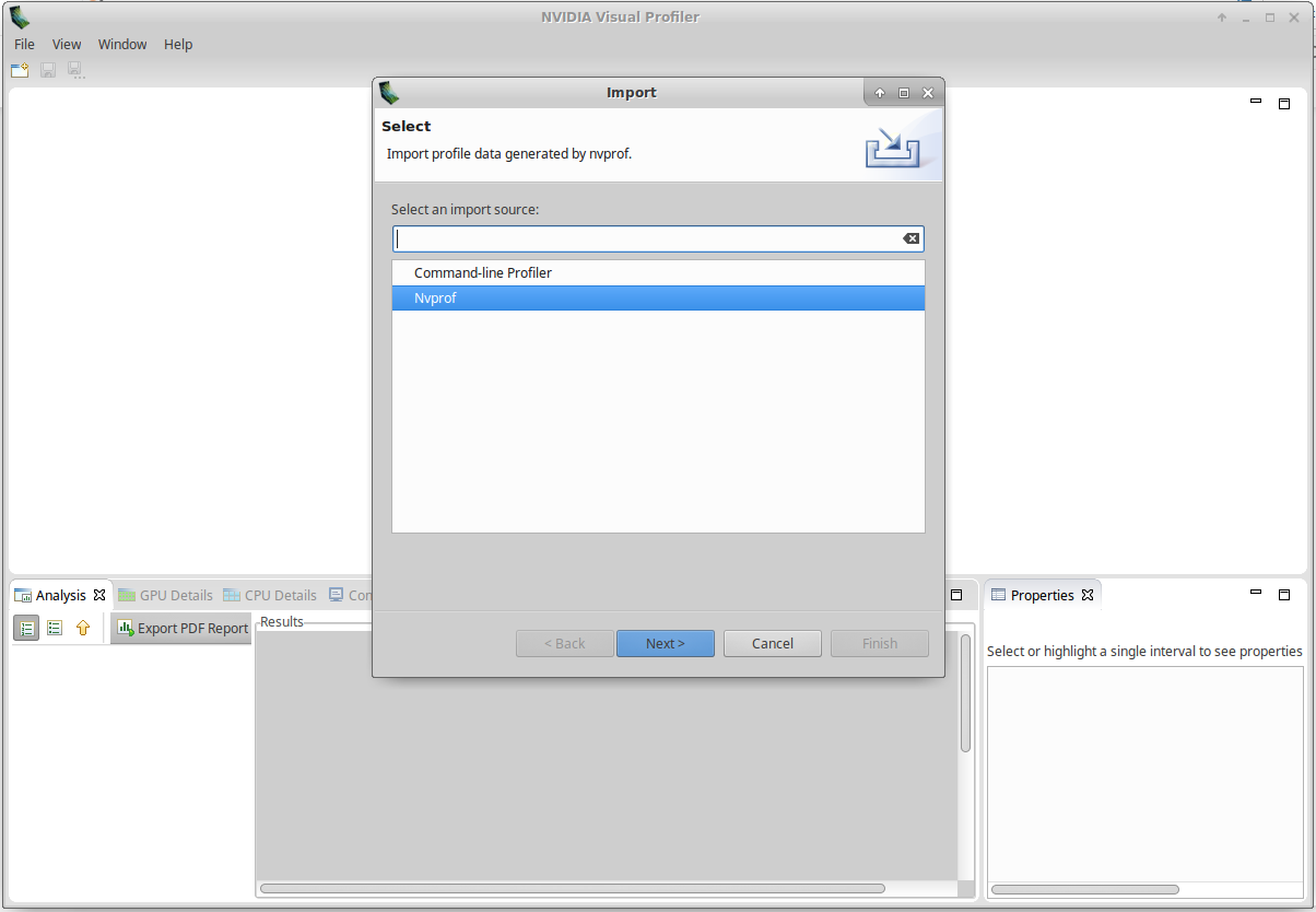
!nvvpClick on File/Import, select Nvprof and click Next:
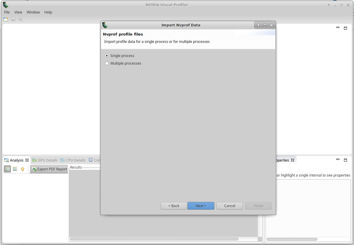
Select Single Process and click Next:
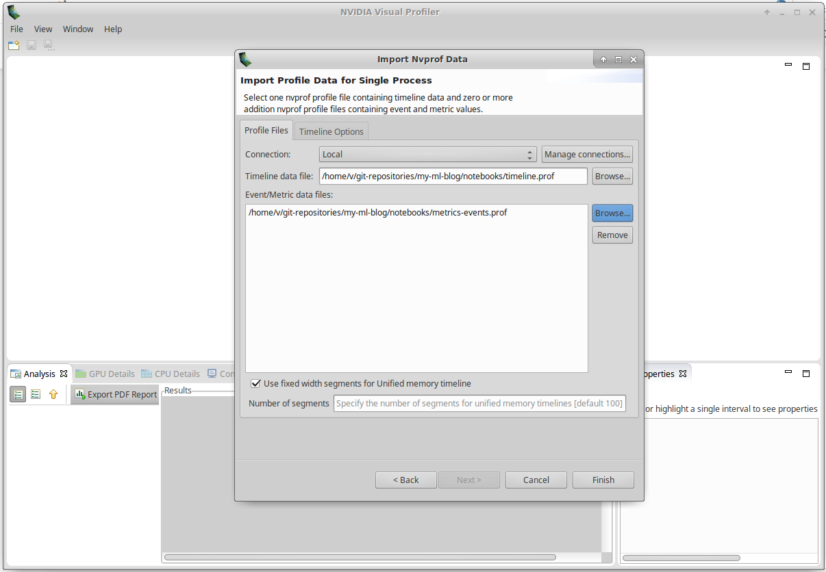
Fill Timeline data file and Event/Metrics data file with the path to your files, and click on Finish:
You should get a screen similar to this:
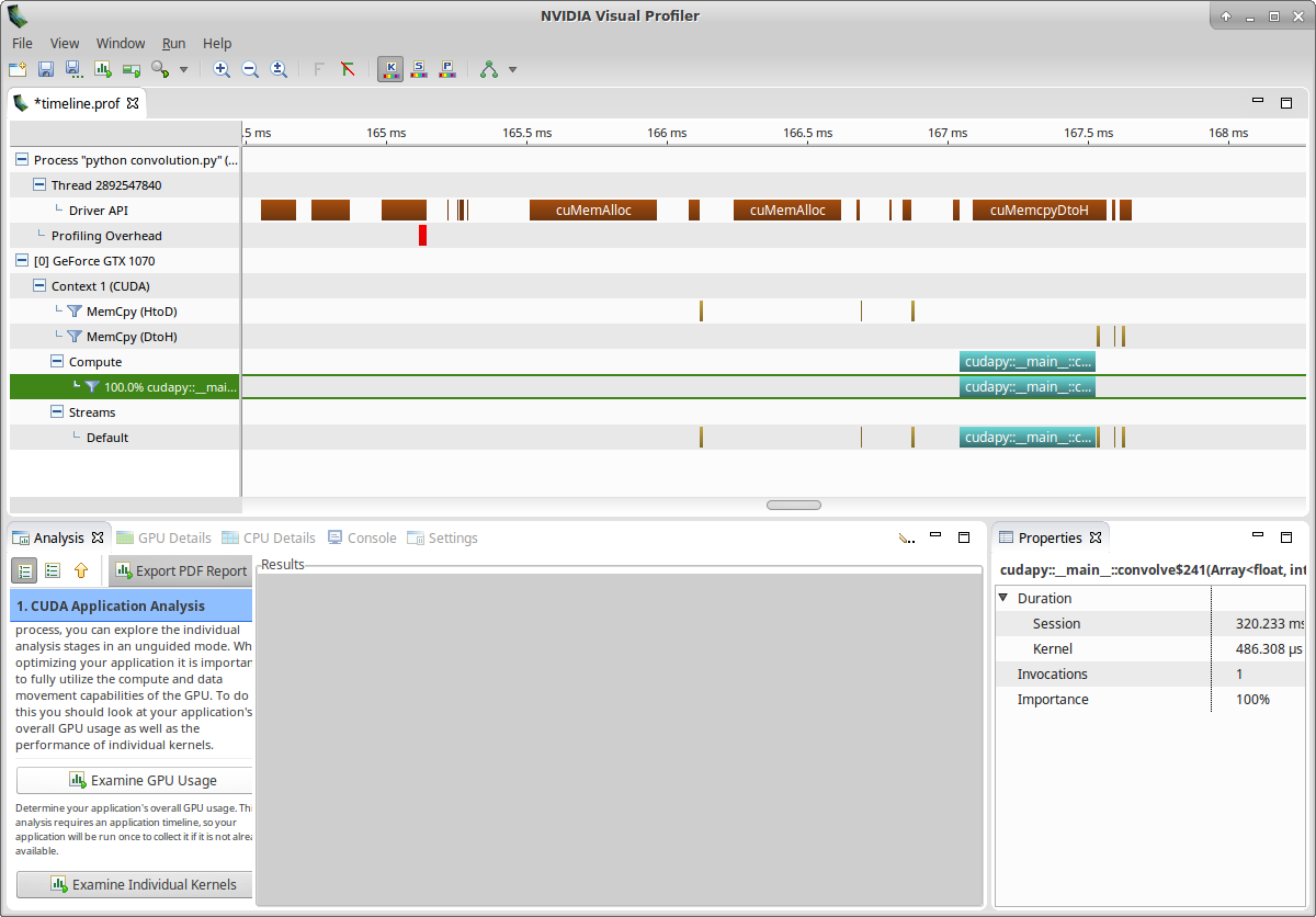
Let’s now examine our kernel:
- Click on Examine Individual Kernels (bottom-left)
- Select the kernel instance (bottom-middle)
- Click on Perform Kernel Analysis (bottom-left)
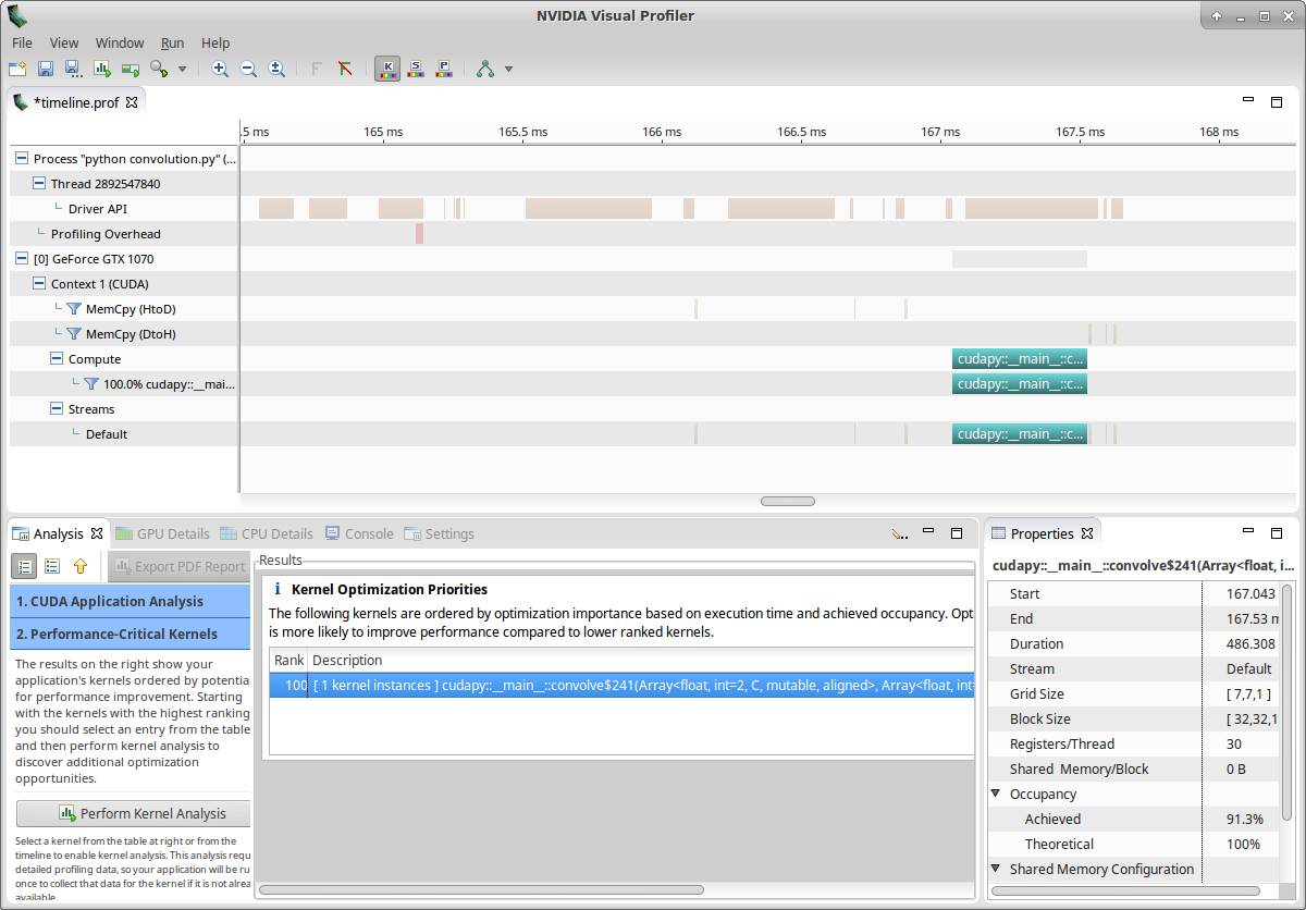
You should get something similar to:
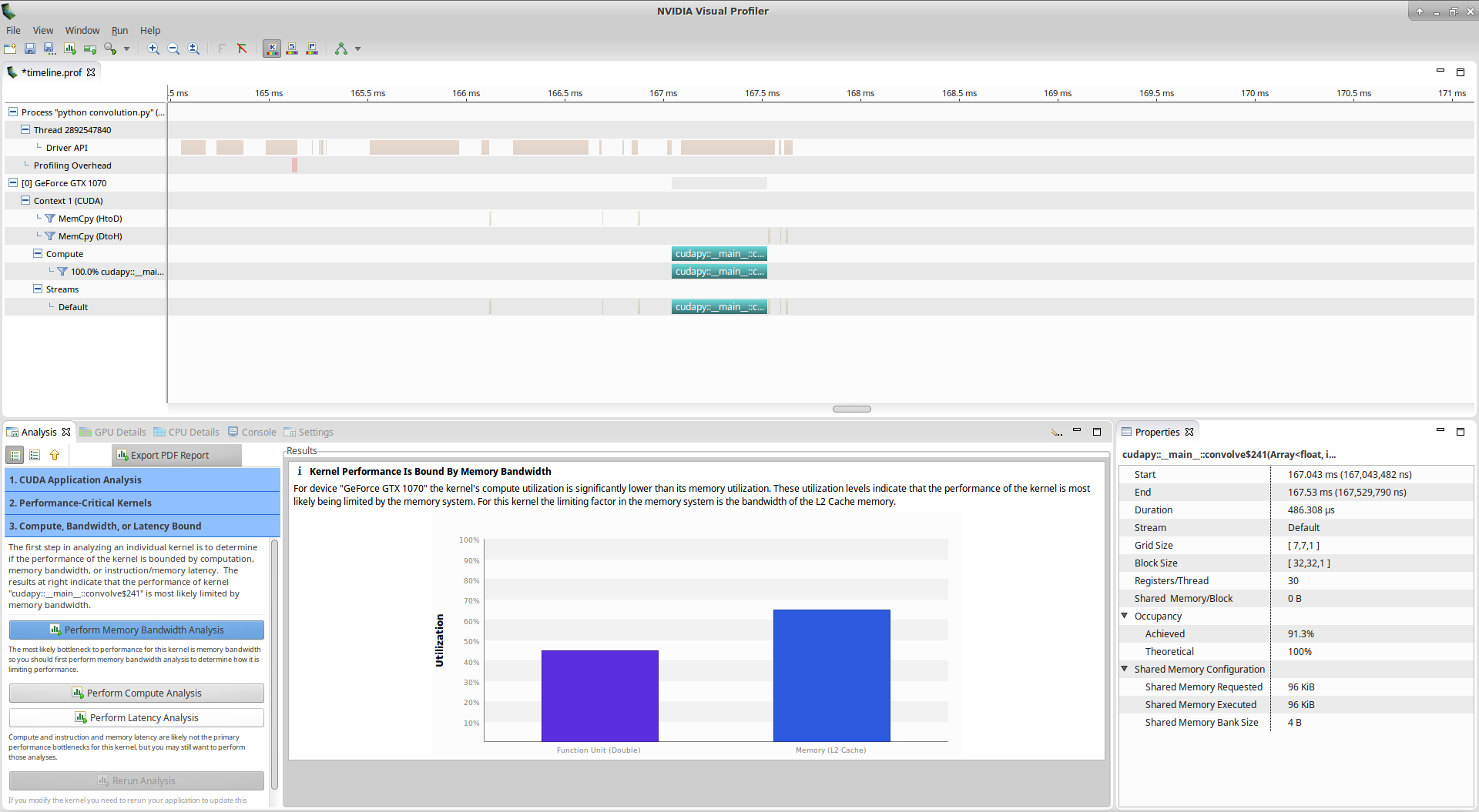
Nvvp tells us that: > Kernel Performance Is Bound By Memory Bandwidth > > For device “GeForce GTX 1070” the kernel’s compute utilization is significantly lower than its memory utilization. These utilization levels indicate that the performance of the kernel is most likely being limited by the memory system. For this kernel the limiting factor in the memory system is the bandwidth of the L2 Cache memory.
However, if you look at the utilization graph, you see that the compute utilization is given as ‘Function Unit(Double)’. Let’s check more details about computation by clicking on Perform Compute Analysis:
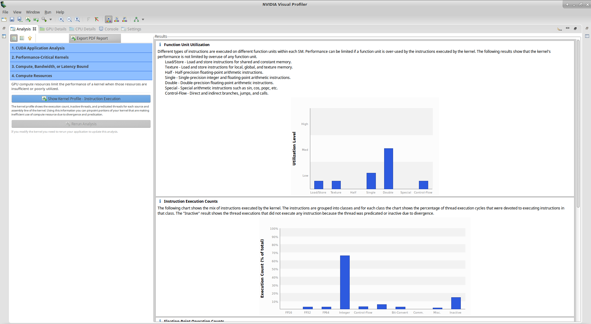
We notice here that the highest Utilization Level is Double. Double means Double-precision floating-point arithmetic instructions. We thought we did all computation in single-precision, that means there is a bug in our kernel!
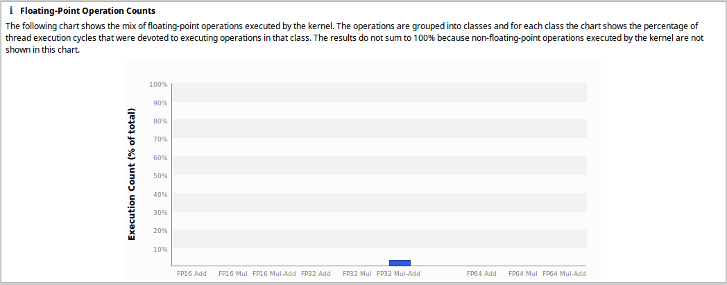
If you look at the Floating-Point Operation Counts section, you see that there is no FP64 Mul but only FP64 Add instructions. This should help us to find the bug easily. In the kernel, additions are made on the line
s += mask[k, l] * image[i_k, j_l].
The problem is that the local variable s is recognized as double while we wanted it to be a single-precision float. The solution is to give a type to s when we initialize it by using: s = numba.float32(0).
When initializing a variable inside a kernel, don’t forget to assign it a type!
Below is a new version of our code taking into consideration this modification:
with open('convolution_nodouble.py', 'r') as f:
    print(f.read())
#!/usr/bin/env python3
# -*- coding: utf-8 -*-
from numba import cuda, float32
import numpy as np
import skimage.data
from skimage.color import rgb2gray
from scipy.ndimage.filters import convolve as scipy_convolve
@cuda.jit
def convolve(result, mask, image):
# expects a 2D grid and 2D blocks,
# a mask with odd numbers of rows and columns, (-1-)
# a grayscale image
# (-2-) 2D coordinates of the current thread:
i, j = cuda.grid(2)
# (-3-) if the thread coordinates are outside of the image, we ignore the thread:
image_rows, image_cols = image.shape
if (i >= image_rows) or (j >= image_cols):
return
# To compute the result at coordinates (i, j), we need to use delta_rows rows of the image
# before and after the i_th row,
# as well as delta_cols columns of the image before and after the j_th column:
delta_rows = mask.shape[0] // 2
delta_cols = mask.shape[1] // 2
# The result at coordinates (i, j) is equal to
# sum_{k, l} mask[k, l] * image[i - k + delta_rows, j - l + delta_cols]
# with k and l going through the whole mask array:
s = float32(0)
for k in range(mask.shape[0]):
for l in range(mask.shape[1]):
i_k = i - k + delta_rows
j_l = j - l + delta_cols
# (-4-) Check if (i_k, j_k) coordinates are inside the image:
if (i_k >= 0) and (i_k < image_rows) and (j_l >= 0) and (j_l < image_cols):
s += mask[k, l] * image[i_k, j_l]
result[i, j] = s
if __name__ == '__main__':
# Read image
full_image = rgb2gray(skimage.data.coffee()).astype(np.float32) / 255
image = full_image[150:350, 200:400].copy()
# We preallocate the result array:
result = np.empty_like(image)
# We choose a random mask:
mask = np.random.rand(13, 13).astype(np.float32)
mask /= mask.sum() # We normalize the mask
# We use blocks of 32x32 pixels:
blockdim = (32, 32)
# We compute grid dimensions big enough to cover the whole image:
griddim = (image.shape[0] // blockdim[0] + 1, image.shape[1] // blockdim[1] + 1)
# We apply our convolution to our image:
convolve[griddim, blockdim](result, mask, image)
# We check that the error with respect to Scipy convolve function is small:
scipy_result = scipy_convolve(image, mask, mode='constant', cval=0.0, origin=0)
max_rel_error = np.max(np.abs(result - scipy_result) / np.abs(scipy_result))
if max_rel_error > 1e-5:
raise AssertionError('Maximum relative error w.r.t Scipy convolve is too large: '
+ max_rel_error)
Let’s execute nvprof in summary mode:
!nvprof python convolution_nodouble.py==31389== NVPROF is profiling process 31389, command: python convolution_nodouble.py
==31389== Profiling application: python convolution_nodouble.py
==31389== Profiling result:
Type Time(%) Time Calls Avg Min Max Name
GPU activities: 88.63% 424.42us 1 424.42us 424.42us 424.42us cudapy::__main__::convolve$241(Array<float, int=2, C, mutable, aligned>, Array<float, int=2, C, mutable, aligned>, Array<float, int=2, C, mutable, aligned>)
5.81% 27.840us 3 9.2800us 704ns 13.568us [CUDA memcpy HtoD]
5.56% 26.624us 3 8.8740us 704ns 13.088us [CUDA memcpy DtoH]
API calls: 98.24% 120.98ms 1 120.98ms 120.98ms 120.98ms cuDevicePrimaryCtxRetain
0.43% 532.97us 1 532.97us 532.97us 532.97us cuLinkCreate
0.38% 473.08us 3 157.69us 12.874us 418.06us cuMemcpyDtoH
0.28% 345.44us 3 115.15us 11.188us 207.94us cuMemAlloc
0.17% 213.41us 1 213.41us 213.41us 213.41us cuModuleLoadDataEx
0.13% 155.91us 1 155.91us 155.91us 155.91us cuLinkAddData
0.11% 130.78us 1 130.78us 130.78us 130.78us cuLinkComplete
0.11% 130.10us 1 130.10us 130.10us 130.10us cuMemGetInfo
0.07% 89.970us 3 29.990us 13.502us 41.667us cuMemcpyHtoD
0.04% 54.566us 1 54.566us 54.566us 54.566us cuDeviceGetName
0.02% 25.161us 1 25.161us 25.161us 25.161us cuLaunchKernel
0.00% 3.8530us 3 1.2840us 357ns 2.2390us cuDeviceGetCount
0.00% 3.2900us 5 658ns 456ns 1.0330us cuFuncGetAttribute
0.00% 2.3000us 1 2.3000us 2.3000us 2.3000us cuCtxPushCurrent
0.00% 1.6720us 2 836ns 771ns 901ns cuDeviceGet
0.00% 1.5600us 3 520ns 416ns 698ns cuDeviceGetAttribute
0.00% 1.4520us 1 1.4520us 1.4520us 1.4520us cuModuleGetFunction
0.00% 906ns 1 906ns 906ns 906ns cuLinkDestroy
0.00% 799ns 1 799ns 799ns 799ns cuDeviceComputeCapability
We see that the kernel is not faster, this is not surprising since it was indicated that the kernel performance was bound by memory bandwidth. We collect the detailed data for further analysis:
!nvprof --quiet --export-profile timeline_nodouble.prof python convolution_nodouble.py
!nvprof --quiet --metrics all --events all -o metrics-events_nodouble.prof python convolution_nodouble.py
We import once again in nvvp and perform compute analysis. In the floating-point operation counts section, we get that only FP32 Mul-Add are used, this is in accordance with our expectations.
In Part 5 of this introduction, we will see how to improve the “performance bounded by memory bandwidth” problem.