An introduction to CUDA in Python (Part 3)

This is the third part of an introduction to CUDA in Python. If you missed the beginning, you are welcome to go back to Part 1 or Part 2.
In this third part, we are going to write a convolution kernel to filter an image.

2D convolution

Since we will be working on images, we will use a 2D grid with 2D blocks. This means that each block is going to work on a small part of the image.

Below is a simple convolution kernel, followed by a few comments:

from numba import cuda
import numpy as np

@cuda.jit
def convolve(result, mask, image):
    # expects a 2D grid and 2D blocks,
    # a mask with odd numbers of rows and columns, (-1-) 
    # a grayscale image
    
    # (-2-) 2D coordinates of the current thread:
    i, j = cuda.grid(2) 
    
    # (-3-) if the thread coordinates are outside of the image, we ignore the thread:
    image_rows, image_cols = image.shape
    if (i >= image_rows) or (j >= image_cols): 
        return
    
    # To compute the result at coordinates (i, j), we need to use delta_rows rows of the image 
    # before and after the i_th row, 
    # as well as delta_cols columns of the image before and after the j_th column:
    delta_rows = mask.shape[0] // 2 
    delta_cols = mask.shape[1] // 2
    
    # The result at coordinates (i, j) is equal to 
    # sum_{k, l} mask[k, l] * image[i - k + delta_rows, j - l + delta_cols]
    # with k and l going through the whole mask array:
    s = 0
    for k in range(mask.shape[0]):
        for l in range(mask.shape[1]):
            i_k = i - k + delta_rows
            j_l = j - l + delta_cols
            # (-4-) Check if (i_k, j_k) coordinates are inside the image: 
            if (i_k >= 0) and (i_k < image_rows) and (j_l >= 0) and (j_l < image_cols):  
                s += mask[k, l] * image[i_k, j_l]
    result[i, j] = s

To simplify a bit the kernel, we will only use masks with odd number of rows and columns.
As seen in Part 2, an easy way to get 2D coordinates is to use the convenience function cuda.grid(2).
We will later divide the image in blocks of \(32 \times 32\) pixels. Note that if we work on an image size that is not a multiple of 32, we have to be careful about the borders. That’s why we check if the thread coordinates are inside the image.
We check if \((i_k, j_k)\) coordinates are inside the image and when they are not, we just ignore the coordinates. This is equivalent to consider that the value of the image is 0 for coordinates outside of it.

Reference image

We are going to test our kernel on the following image:

import skimage.data
from skimage.color import rgb2gray

%matplotlib inline
import matplotlib.pyplot as plt

full_image = rgb2gray(skimage.data.coffee()).astype(np.float32) / 255
plt.figure()
plt.imshow(full_image, cmap='gray')
plt.title("Full size image:")
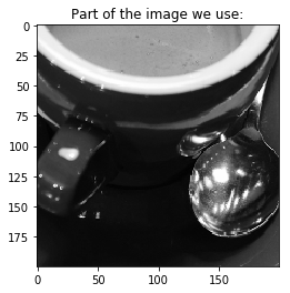
image = full_image[150:350, 200:400].copy() # We don't want a view but an array and therefore use copy()
plt.figure()
plt.imshow(image, cmap='gray')
plt.title("Part of the image we use:")
plt.show()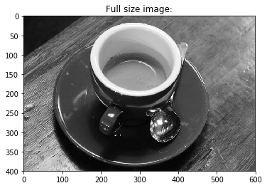

png

Running the kernel

Let’s now try our kernel:

# We preallocate the result array:
result = np.empty_like(image)

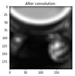
# We choose a random mask:
mask = np.random.rand(13, 13).astype(np.float32) 
mask /= mask.sum()  # We normalize the mask
print('Mask shape:', mask.shape)
print('Mask first (3, 3) elements:\n', mask[:3, :3])

# We use blocks of 32x32 pixels:
blockdim = (32, 32)
print('Blocks dimensions:', blockdim)

# We compute grid dimensions big enough to cover the whole image:
griddim = (image.shape[0] // blockdim[0] + 1, image.shape[1] // blockdim[1] + 1)
print('Grid dimensions:', griddim)

# We apply our convolution to our image:
convolve[griddim, blockdim](result, mask, image)

# We plot the result:
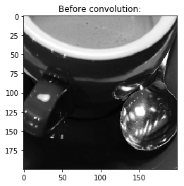
plt.figure()
plt.imshow(image, cmap='gray')
plt.title("Before convolution:")
plt.figure()
plt.imshow(result, cmap='gray')
plt.title("After convolution:")
plt.show()

Mask shape: (13, 13)
Mask first (3, 3) elements:
 [[0.00663321 0.00477909 0.0041353 ]
 [0.00323536 0.00892652 0.00866179]
 [0.00715392 0.00091124 0.00370887]]
Blocks dimensions: (32, 32)
Grid dimensions: (7, 7)

png

Checking the result

Let’s check that our convolution kernel returns the correct result:

from scipy.ndimage.filters import convolve as scipy_convolve

scipy_result = scipy_convolve(image, mask, mode='constant', cval=0.0, origin=0)
print('Maximum relative error:', np.max(np.abs(result - scipy_result) / np.abs(scipy_result)))

Maximum relative error: 1.1916778e-07

OK, there is no big difference between the two results!

Timing

Let’s time our kernel:

%timeit convolve[griddim, blockdim](result, mask, image)

1.2 ms ± 6.02 µs per loop (mean ± std. dev. of 7 runs, 1000 loops each)

and compare the result with scipy convolution:

scipy_result = np.empty_like(image)
%timeit scipy_convolve(image, mask, output=scipy_result, mode='constant', cval=0.0, origin=0)

6.5 ms ± 9.69 µs per loop (mean ± std. dev. of 7 runs, 100 loops each)

Our kernel is \(5\times\) faster when taking into consideration the memory transfers between host and device.

d_image = cuda.to_device(image)
d_mask = cuda.to_device(mask)
d_result = cuda.to_device(result)
%timeit convolve[griddim, blockdim](d_result, d_mask, d_image)

210 µs ± 48.9 µs per loop (mean ± std. dev. of 7 runs, 1 loop each)

Our kernel is \(30\times\) faster when considering the computation on device only.

In Part 4 of this introduction, we will see how to profile a CUDA kernel using NVIDIA tools.